Sensing
A LiDAR spins a laser and times each bounce, giving a ring of distances. Cameras, sonar, and depth sensors do similar jobs.
Every reading is a little wrong. Noise is normal, not a bug.
Engineering · Robot Autonomy · Perception
Imagine waking up in a dark room you have never seen. Where are the walls? Where are you? Robots have to answer both questions at the same time. Help a robot draw a map with laser “flashlights,” then make your own map of the classroom with a tape measure.
A robot dropped into a new building knows nothing: not where the walls are, and not where it is. Every self-driving car, warehouse robot, and robot vacuum has to answer two questions at once — what does the world look like? and where am I in it? Build a map from laser scans, then recreate the experiment with an ELEGOO ultrasonic sensor or a tape measure. Watch position errors distort a map and use a cloud of guesses to find a lost robot.
← Back to EngineeringExplorer · Story time
I’m Bolt. When I roll into a new room, I can’t see like you. Instead, I shine invisible laser beams all around me, like lots of tiny flashlights. Each beam tells me how far away the wall is.
Every place a beam goes through must be empty floor. The place where it stops must be a wall. I color my map one square at a time: white for floor, black for wall, gray for “I don’t know yet.”
But here is the tricky part. My wheels slip a little, so I’m never totally sure where I am. If I get my place wrong, my map gets smeary!
The big idea
If a robot had a perfect map, it could figure out where it is by comparing what its sensors see against the map. That is localization. If it knew exactly where it was at every moment, it could build a map by recording what its sensors see from each spot. That is mapping. In an unknown place it has neither — so it must do both at once. Engineers call that SLAM: Simultaneous Localization And Mapping.
A LiDAR spins a laser and times each bounce, giving a ring of distances. Cameras, sonar, and depth sensors do similar jobs.
Every reading is a little wrong. Noise is normal, not a bug.
Odometry counts wheel turns (encoders) and measures turning (a gyro) to estimate how far the robot moved.
Tiny errors add up. After a few laps, the robot's belief can be meters off.
An occupancy grid splits the floor into cells. Each cell stores the probability it is blocked, starting at "no idea."
This grid is exactly what a planner like A* searches.
Classroom fieldwork
Start with a tabletop room made from upright cardboard walls. Mark a sensor station on graph paper, then measure distances in several directions. You can reproduce the key ideas without buying a LiDAR or building a driving robot.
20–30 minutes · No electronics. Students act as sensor, mapper, and position tracker. Best first encounter with free, occupied, and unknown space.
45–60 minutes after setup · UNO R3, HC-SR04, optional positional servo. Collect real echoes and plot them in the scan notebook below.
One extra class · Stop at marked stations and scan. Compare measured position with a motion estimate to reveal drift.
What we are modeling: these activities use known or manually measured sensor positions. They demonstrate mapping and localization separately; they do not run a complete SLAM algorithm. Ultrasound spreads into a cone, so its echoes are less precise in direction than the sim’s laser rays.
Gather: graph paper, ruler or tape measure, protractor, pencil, cardboard walls, and three colored pencils. Work in teams of three: sensor operator, mapper, and checker. Use a 10 cm grid for a tabletop room or a larger taped floor grid.
DIY variations: rotate a ruler around a paper protractor for a tiny desk model, or use taut string and a tape measure for a floor map. Keep students’ eyes open; the mapper can face away from the room and receive only angle/distance reports.
Gather: a 5 V UNO R3-compatible board (such as ELEGOO), USB cable, HC-SR04 ultrasonic module, breadboard, jumper wires, cardboard walls, and a protractor. Optional: an SG90-style positional servo and a regulated 5 V servo supply. Check your kit inventory; not every ELEGOO kit contains these parts.
Mount the sensor level with the walls. Tape its base down at a known station. Start with large, flat targets 20–100 cm away; keep fabric and narrow table legs out of the first test. Aim from the midpoint between the two transducers.
| Component lead | Connect to | Reason |
|---|---|---|
| HC-SR04 VCC / GND | UNO 5 V / GND | Sensor power and reference |
| HC-SR04 TRIG / ECHO | D7 / D8 | Send a pulse / time the returning echo |
| Servo signal (often orange/yellow) | D9 | Command the scan angle |
| Servo + (often red) | External regulated 5 V + | Supply rated for the servo’s current |
| Servo ground (often brown/black) | Supply − and UNO GND | All grounds share a reference |
Disconnect power while wiring. Check pin labels and servo documentation rather than trusting wire color. Do not connect the external supply’s positive lead to the UNO 5 V pin while USB powers the board. An HC-SR04’s 5 V ECHO must be level-shifted for a 3.3 V board. This wiring and sketch are for a standalone UNO, not a robot-car shield.
classroom-sonar, open it in Arduino IDE, choose the UNO board and port, and upload. It uses the standard Servo library.REVERSE_ANGLE = true. Avoid the servo’s mechanical stops.USE_SERVO = false. Place the sensor over a protractor; the sketch prompts for each angle. Turn it by hand and send n when ready.s to take one scan. Compare the 90° reading with a ruler at 20, 50, and 100 cm. Repeat three times and record the spread before mapping.NA means unknown; never turn a timeout into a zero-distance wall.Echo math: distance in cm ≈ echo time in microseconds × 0.0343 ÷ 2. We divide by two because the sound travels to the object and back. The sketch waits at least 65 ms between pings and accepts 2–200 cm for this classroom experiment.
Troubleshoot: repeated NA → check pins, common ground, and a broad flat target. Board resets or a jittering servo → check the servo supply. Slanted walls can reflect sound away; cloth can weaken echoes. Two sensors pinging together can interfere, so run one station at a time or stagger scans.
Build support: ELEGOO kit downloads, Arduino servo wiring and power, and Arduino echo pulse timing.
Gather: your assembled ELEGOO car or DIY chassis with a distance sensor, a taped course, ruler, and paper heading marks. Use the manufacturer’s example to verify the sensor and motors first. Car versions use different shields and pin assignments; do not upload the standalone scanner sketch unchanged.
Extensions: wheel encoders estimate distance from turns (distance ≈ turns × wheel circumference); compare against a ruler to reveal slip. An IMU can help estimate turning, but a gyro’s bias also drifts. A line sensor can detect a taped checkpoint; it does not measure the distance to a room wall.
Limit: motor-on time is only a rough motion estimate, not measured wheel odometry. Autonomous SLAM needs a pose estimator and repeated scan matching or another correction method. Use ELEGOO’s V4.0 documentation only if that is your car version; find other versions in the download center.
From measurement to map
Paste a sensor scan or type tape-measure readings. Set the pose (position + heading) where the scan was taken, then add it to the plot. Add a second scan to see whether the walls line up. This draws measured endpoints and approximate beam paths, not a probabilistic occupancy grid.
Blue = first scan · orange = later scans · dot = possible surface · line = approximate sound path. Blank areas remain unknown.
| Scan | Angle ° | Range cm | Endpoint x | Endpoint y |
|---|
Try a position error: add the example at x = 300. Change x to 325 and add the same readings again. The surfaces separate by 25 cm although the readings did not change. Clear the notebook and repeat with scans from two measured stations.
Math bridge: endpoint x = sensor x + distance × cos(heading + scan angle); endpoint y = sensor y + distance × sin(heading + scan angle). Convert degrees to radians when using code. A sonar echo can come from anywhere within its beam; the endpoint dot is a convenient approximation, not a pinpoint measurement.
Localization you can hold
Draw a known room map and mark four possible sensor stations with the same heading. The teacher chooses one and reports three tape-measure or sonar distances. Put a counter at every candidate station; predict the three readings from each position.
Exit ticket: submit two scans with pose labels, a map showing free/occupied/unknown space, one repeated-measurement comparison, and a sentence explaining whether your activity performed mapping, localization, or full SLAM.
Sim 1 · Occupancy grid mapping
The robot wanders and scans ten times a second. Along each laser ray, cells the beam passed through get a vote for "free"; the cell where it stopped gets a vote for "wall." Votes add up, so one noisy reading can't ruin the map — but many consistent readings make a cell nearly certain. Click anywhere to send the robot there.
Keyboard: Tab into the map, move the crosshair with ←↑→↓ (Shift for bigger steps), and press Enter to send the robot.
Drop the beams to 4. How long does the map take now? Then crank the noise to 25. Do the walls get fuzzier or just slower to appear?
Turn on drifting odometry. The orange robot is where the robot believes it is. Its map is drawn from that belief — watch the walls double and smear.
The laser readings were fine in both runs. Why did the map still break? What would the robot need to notice to fix itself?
Sim 2 · Particle filter
Now flip the problem: the robot has the map but has no idea where it is. A particle filter scatters hundreds of guesses (red dots) across the map. Each cycle it does three things:
Survival of the fittest guess. The yellow robot appears once the cloud agrees.
Keyboard: same as the mapping sim. Arrows move the crosshair, Enter sends the robot.
Small σ trusts the laser completely; big σ shrugs at mismatches.
Early on, the cloud often splits into two or three clumps. Those are places that look the same to the laser. Which rooms in the map are twins?
Press Kidnap robot with random guesses on, then again with them off. Why can't a filter with no fresh guesses recover?
Set σ to 4. The cloud collapses fast — sometimes onto the wrong spot. Overconfidence is a real engineering failure.
Engineer deep dive
Each cell stores ℓ = log( p / (1 − p) ). Bayes' rule for independent readings then becomes plain addition:
ℓt = ℓt−1 + log( p(occ | z) / p(free | z) ) − ℓ0
That is why the sim's map “votes”: a hit adds +0.9, a pass-through adds −0.4, and ℓ is clamped to ±5. The clamp keeps a cell able to change its mind when furniture moves.
bel⁻(xt) = ∫ p(xt | ut, xt−1) bel(xt−1) dxt−1
bel(xt) = η · p(zt | xt) · bel⁻(xt)
A Kalman filter solves this exactly when everything is Gaussian. A particle filter approximates bel with N weighted samples, so it can hold the multi-modal belief you see when the cloud splits into clumps.
With B beams, each predicted range r̂k and measured rk:
w ∝ Πk exp( −(rk − r̂k)² / 2σ² )
Multiply 12 small numbers and you underflow fast, so real code sums log-weights. Small σ makes the product razor-sharp. That is the overconfidence you see at σ = 4.
Modern SLAM (graph SLAM, factor graphs) stores every pose as a node and every odometry step or scan match as a spring between nodes. Loop closure adds one more spring, and a least-squares solver relaxes the whole graph at once. Libraries like g2o, GTSAM, and Cartographer do this in real time.
Putting it together
Sim 1 showed that mapping with a drifting position ruins the map. Sim 2 showed that matching scans to a map fixes the position. SLAM does both in a loop: it uses the map-so-far to correct its position, then uses the corrected position to extend the map.
Slide the new scan around until it lines up with the map built so far. The shift needed is the odometry error — subtract it.
When the robot returns somewhere it has been and recognizes it, it knows its whole path must bend to meet up. The entire map snaps straight.
Robot vacuums (LiDAR on top), Mars rovers, VR headsets tracking your room, phone AR apps, and self-driving cars all run some form of SLAM.
Next → Sensor Fusion: combine noisy wheels, gyros, and accelerometers into one good estimate
Where you’ll see it
Click any photo to enlarge it.
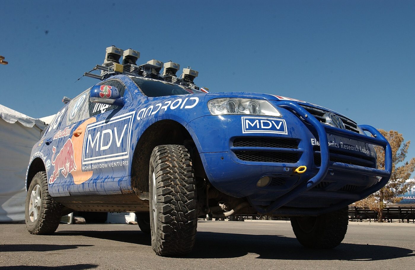
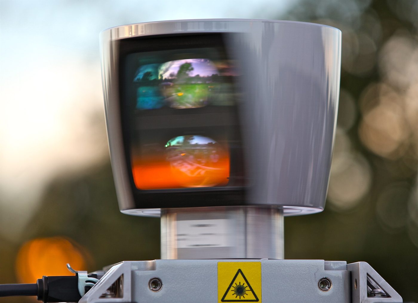
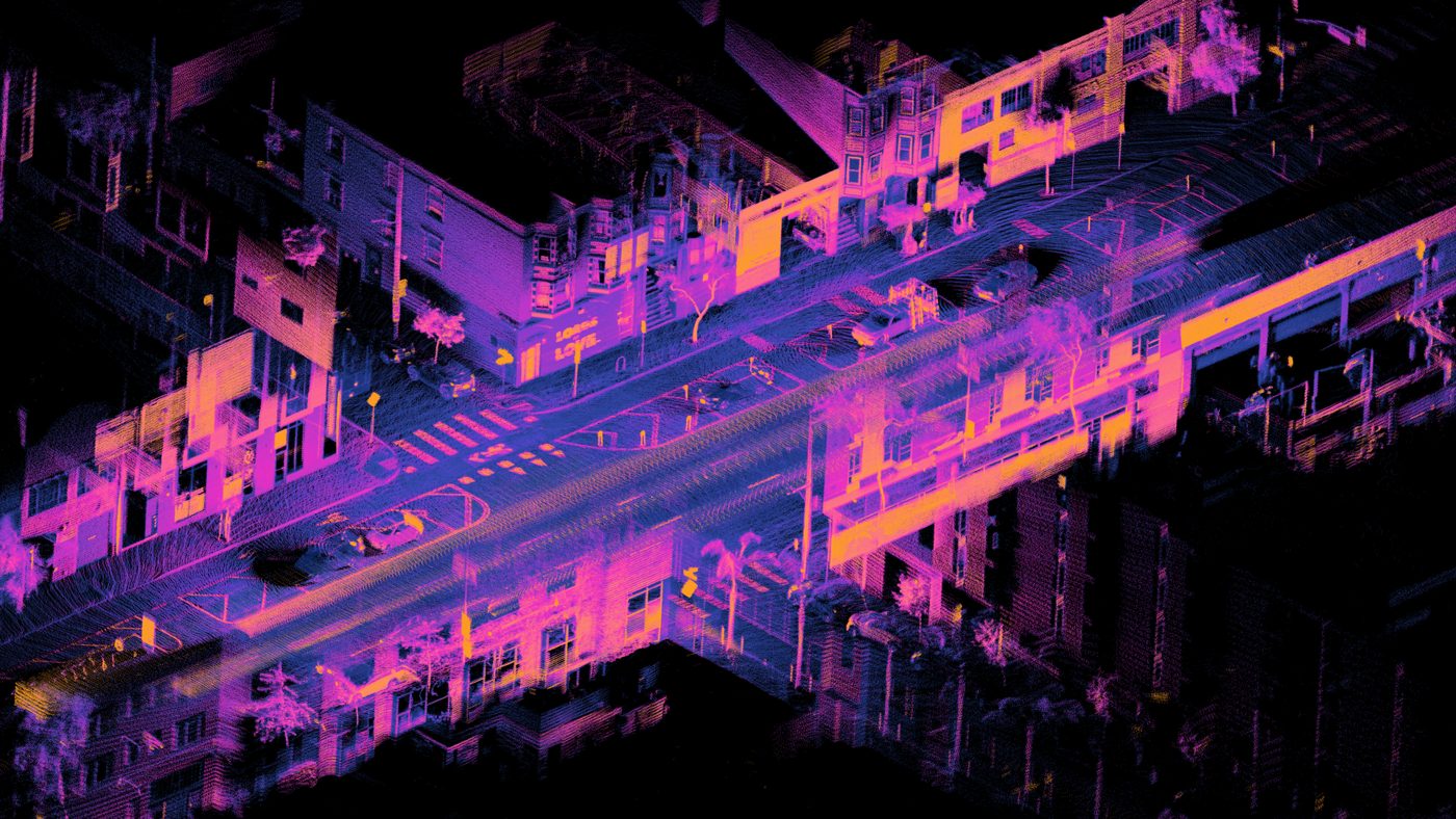
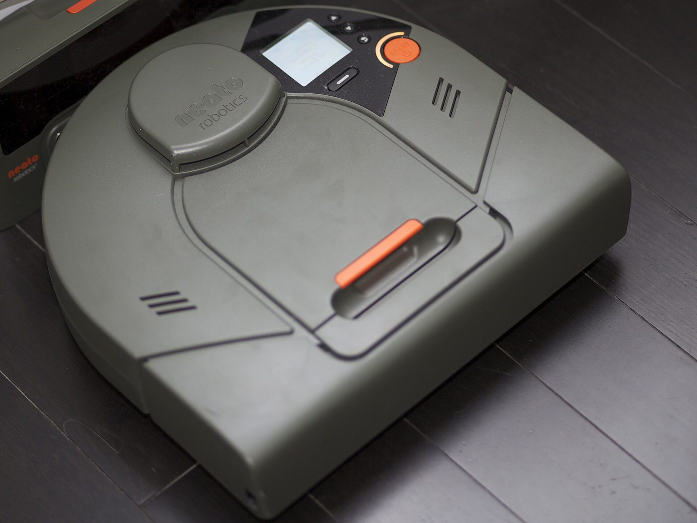
Robot autonomy series
Quick check
1. A laser beam goes all the way across a square without stopping. What is that square?
2. Why does the map get smeary when the robot's wheels slip?
3. On the robot's map, what does gray mean?
1. Why is SLAM called a chicken-and-egg problem?
2. A laser beam travels 3 m before hitting a wall. What do the cells along the first 3 m get?
3. Why does odometry drift get worse over time?
4. In a particle filter, which guesses get copied most during resampling?