Focus on left, right, middle, more, less, most common, and simple tally charts. Students predict with words before seeing data.
Mathematics · Probability Distributions & Expected Value
Galton Board & Pachinko Lab
A Galton board is a beautiful probability machine: each peg nudges a ball left or right, and many tiny decisions add up to a visible distribution. Part 2 of the probability sequence: the Probability Simulator studies one coin or die at a time; this lab adds many of those events together and watches a bell curve appear. It moves beyond coins and dice into systems thinking, showing how sample size, bias, design choices, expected value, and data displays can change what students believe about chance.
← Back to MathematicsLesson Launchpad
This lesson treats pachinko as an engineering and probability case study. Students study the path of a ball through pegs, then use the simulator to make predictions, collect data, and explain why the center bins usually fill more than the edges on a fair board.
Students Should Leave Able To
- connect a pachinko board to repeated left-right probability events.
- explain why a fair board often forms a mound-shaped distribution.
- describe how Francis Galton used the board to show the bell curve emerging from many random events.
- describe how bias, obstacles, and board geometry change outcomes.
- compare experimental counts with an expected model.
- use simulations ethically by separating amusement history from mathematical analysis.
5-Minute Start
- 1Ask students where one ball is most likely to land: edge, center, or impossible to predict.
- 2Run 100 balls on the fair board and let students describe the shape before naming it.
- 3Run 2000 balls, turn on the bell curve, and introduce "many small random choices can create a stable pattern."
Use fractions, percentages, bar graphs, sample size, and fair-versus-biased comparisons. Students explain why center bins have more paths.
Connect binomial probability, expected value, weighted outcomes, variance, normal approximation, and model limitations.
Interactive Lab
Run the Pachinko Simulator
Choose a board scenario, change the number of peg rows, and launch a sample. The yellow markers show the expected model; the blue bars show what happened in this run. Turn on the bell curve to compare the bins with the smooth normal curve Galton predicted.
Current model A fair board uses the same probability for left and right at every peg. The center bins have more possible paths, so they are expected to fill more often.
Trials
0
Most Common
--
Mean Bin
--
Center Share
--
Bin Distribution
Launch a sample to compare the expected model with experimental results.
The Galton Board: Where the Bell Curve Comes From
The simulator above is a digital Galton board. Sir Francis Galton (1822–1911), an English scientist, built one in the 1870s to show how the normal distribution arises. He described it in his 1889 book Natural Inheritance. He called it a quincunx, after the five-dot pattern on a die, because the pins sit in staggered rows: each pin is centered under the gap between two pins above it.
In this model, each ball makes a string of independent left-or-right choices with the same probability at every row. The landing bin follows a discrete binomial distribution. On a fair board with many rows, that shape can be approximated by a smooth normal curve; a small sample may still look lumpy.


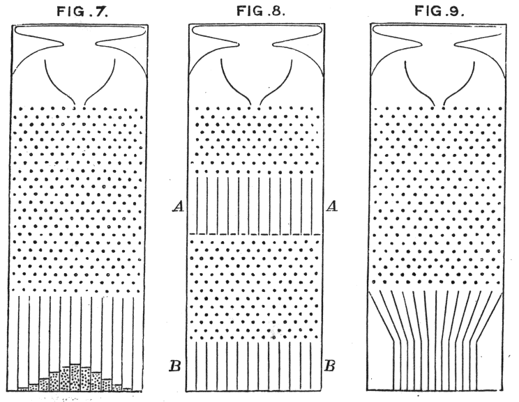


The big idea: the central limit theorem
Each landing bin counts the rightward choices across a fixed number of rows. If those choices are independent and each has the same probability, the count is binomial. With enough rows and probabilities away from 0 and 1, a normal curve is a useful approximation. Real-world data need their own evidence before we call them normal. See OpenStax's normal-approximation conditions.
On the fair board, run 50 balls, then 3000. Compare the bins to the green bell curve. The small run is lumpy; the big run hugs the curve.
Set 6 rows, then 14. More rows means each ball adds up more bounces, and the bins fit the bell curve more closely.
One ball is unpredictable. Thousands of balls are very predictable. How can both be true at the same time?
- Teacher background: Francis Galton, Natural Inheritance (1889), chapter 5; Galton board and central limit theorem on Wikipedia.
Pachinko History, K-12 Framing
Pachinko is the arcade cousin of Galton's board. It grew from earlier peg-and-ball amusements such as bagatelle and the Corinth game, which reached Japan in the early 1900s. By the 1930s, pachinko had become associated with amusement halls in Nagoya and later developed into a major Japanese entertainment industry after World War II.
Classroom boundary
In this lesson, pachinko is studied as a mechanical design and probability system. Keep discussion focused on culture, engineering, statistics, and responsible analysis rather than gambling behavior.
Peg boards, spring launches, and gravity created a family of games where motion and chance are inseparable.
The spacing of pins, the launch speed, and the slope of the board all affect the path of a ball.
Pachinko machines became a recognizable part of urban entertainment, especially in the postwar period.
- Teacher background: Daikoku Denki history timeline and Pachinko Industry Web Reference.
Simulation Scenarios
Each scenario is a classroom investigation, not just a setting. Have students predict first, run the model, then write one sentence connecting the data to a math concept.
Run 50 balls, then 3000. Students should notice that larger samples usually look smoother and closer to the expected model.
Count how many left-right paths reach each bin. The center has many path combinations; the far edge has only one all-left or all-right path.
Use left or right bias. Students decide whether the evidence is strong enough to claim the board is unfair.
Assign point values to bins on paper and multiply each value by its probability. The "best-looking" target may not be the best expected outcome.
Compare the center-friendly scenario to the fair board and discuss how design can steer outcomes without removing randomness.
Ask how a graph could exaggerate differences. Students should inspect scales, sample size, and whether expected values are shown.
Teach the Math
Independent events: In the simplest model, each peg collision is treated as a new left-or-right event. The previous bounce does not force the next bounce to compensate.
Binomial distribution: If a board has 10 rows, the ball makes 10 left-right decisions and lands in one of 11 bins. The number of right bounces determines the bin.
Normal approximation: With enough independent rows and a right-bounce probability away from 0 or 1, the binomial shape can be approximated by a normal curve with mean np and standard deviation √(np(1 − p)). On a fair 10-row board, the mean is 5 and the standard deviation is about 1.58; the discrete bin probabilities give the exact answer. The 68–95–99.7 rule in How Spread Out? describes a continuous normal model.
Expected value: If bins have point values, multiply each bin's value by its probability and add the results. Expected value is a long-run average, not a promise for one ball.
The pattern of counts across all possible outcomes.
The bin or outcome that appears most often in a data set.
A systematic tilt in a process that makes some outcomes more likely than the fair model predicts.
Random outcomes are not automatically balanced in small samples. Pattern and variation can exist at the same time.
Suggested Lesson Sequence
Show the board and ask students to point to the bin they think will win. Do not reveal the expected model yet.
Run a fair sample and compare the center with the edges. Name the binomial pattern.
Groups investigate a different board setting and write a claim-evidence-reasoning paragraph.
Students decide which board is fairest, which is most predictable, and which is hardest to model.
Explain why a center bin can be most likely even though each peg only gives two choices.
Discussion Prompts
How many different paths can reach an edge bin? How many can reach a middle bin?
Galton called the board a quincunx. Why do the pins have to be staggered? What would happen if every pin sat directly under the one above?
When does a weird result mean "random variation," and when might it be evidence of bias?
How would you design a pachinko board to make outcomes more predictable?
Why should a simulator show both experimental data and an expected model?
What parts of the real world are missing from this model: friction, spin, ball size, peg shape, or human launch force?
How can probability knowledge help people make better decisions around games, risk, and advertising?